
tf.keras.applications.VGG16
- fine tuning
- 모델이 10개 밖에 없다.
keras에 applications를 통해 유명한 모델들을 가져올 수 있습니다. keras에서 가져올수 있는 모델들로는 다음과 같습니다.
- Xception
- VGG16
- VGG19
- ResNet, ResNetV2
- InceptionV3
- InceptionResNetV2
- MobileNet
- MobileNetV2
- DenseNet
- NASNet
from tensorflow.keras.applications import VGG16

vgg = VGG16(include_top=False, weights ='imagenet')
# include_top이 False이면 Dense(Fully connected layer)를 집어넣지 않는다.
vgg.summary()
'''
Model: "vgg16"
_________________________________________________________________
Layer (type)                 Output Shape              Param #
=================================================================
input_2 (InputLayer)         [(None, None, None, 3)]   0
_________________________________________________________________
block1_conv1 (Conv2D)        (None, None, None, 64)    1792
_________________________________________________________________
block1_conv2 (Conv2D)        (None, None, None, 64)    36928
_________________________________________________________________
block1_pool (MaxPooling2D)   (None, None, None, 64)    0
_________________________________________________________________
block2_conv1 (Conv2D)        (None, None, None, 128)   73856
_________________________________________________________________
block2_conv2 (Conv2D)        (None, None, None, 128)   147584
_________________________________________________________________
block2_pool (MaxPooling2D)   (None, None, None, 128)   0
_________________________________________________________________
block3_conv1 (Conv2D)        (None, None, None, 256)   295168
_________________________________________________________________
block3_conv2 (Conv2D)        (None, None, None, 256)   590080
_________________________________________________________________
block3_conv3 (Conv2D)        (None, None, None, 256)   590080
_________________________________________________________________
block3_pool (MaxPooling2D)   (None, None, None, 256)   0
_________________________________________________________________
block4_conv1 (Conv2D)        (None, None, None, 512)   1180160
_________________________________________________________________
'''
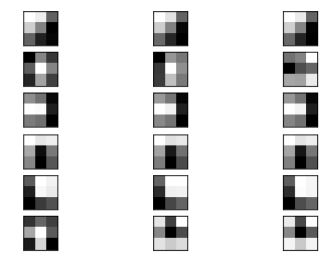
Filter Visualization
불러온 모델에서 특정 레이러를 뽑아낼 수 있습니다. 각 레이어마다 고유의 bias와 filters가 있습니다.
get_layer를 이용해서 뽑아낼 수 있고, get_weights()를 가져올 수 있습니다.
block1_conv1 = vgg.get_layer('block1_conv1')

# vgg.layers[1].get_weights()
filters, bias = block1_conv1.get_weights()
filters.shape
# (3, 3, 3, 64)

bias.shape
# (64,)

filters[...,0].shape
# (3, 3, 3)

import matplotlib.pyplot as plt
n_filters, ix = 6, 1
for i in range(n_filters):
	# Get the filter
	f = filters[:, :, :, i]
	# Plot each channel separately
	for j in range(3):
		# Specify subplot and turn of axis
		ax = plt.subplot(n_filters, 3, ix)
		ax.set_xticks([])
		ax.set_yticks([])
		# Plot filter channel in grayscale
		plt.imshow(f[:, :, j], cmap='gray')
		ix += 1
keras: VGG16
# 남이 만든 모델 (학습된 모델)
from tensorflow.keras.applications import VGG16
from tensorflow.keras.applications.vgg16 import preprocess_input
from tensorflow.keras.preprocessing.image import load_img
from tensorflow.keras.preprocessing.image import img_to_array
import numpy as np
from tensorflow.keras.models import Model
- layer 선택해서 feature 뽑아 보기
vgg = VGG16()
model = Model(inputs=vgg.inputs,
              outputs=vgg.layers[2].output)
model.summary()
'''
Model: "model_1"
_________________________________________________________________
Layer (type)                 Output Shape              Param #
=================================================================
input_2 (InputLayer)         [(None, 224, 224, 3)]     0
_________________________________________________________________
block1_conv1 (Conv2D)        (None, 224, 224, 64)      1792
_________________________________________________________________
block1_conv2 (Conv2D)        (None, 224, 224, 64)      36928
=================================================================
Total params: 38,720
Trainable params: 38,720
Non-trainable params: 0
_________________________________________________________________
'''
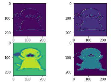
- features 뽑을 데이터 로드
VGG와 같이 모델을 불러와서 사용할 때, 데이터의 shape를 맞춰줘야 합니다. 여기서는 (1,224,224,3) 으로 맞춰줘야하기 때문에 데이터를 resize 해주도록 하겠습니다.
import PIL
bono = PIL.Image.open('bono.jpg')
# 사이즈를 바꿔준다.
bono = bono.resize((224,224))
# np.array로 바꿔준다.
img = img_to_array(bono)

img = np.expand_dims(img,axis=0)
# [np.newaxis]

# 모델(VGG, etc) 전처리 방법을 같이 적용
img=preprocess_input(img)

# VGG 학습
feature_maps = model.predict(img)

fig, axes=plt.subplots(2,2)
for i,axs in enumerate(axes.ravel()):
    axs.imshow(feature_maps[0,...,i])
Tensorflow hub (Transfer learning)
- feature url: fc(fully-connected) layer가 없습니다.
- classification url: 모델 전체를 가져온 것 - include_top= False
- layer가 한개밖에 없어서 fine tuning 못한다.
-
Feature Extraction: Use the representations learned by a previous network to extract meaningful features from new samples. You simply add a new classifier, which will be trained from scratch, on top of the pretrained model so that you can repurpose the feature maps learned previously for our dataset.
You do not need to (re)train the entire model. The base convolutional network already contains features that are generically useful for classifying pictures. However, the final, classification part of the pretrained model is specific to original classification task, and subsequently specific to the set of classes on which the model was trained.
-
Fine-Tuning: Unfreezing a few of the top layers of a frozen model base and jointly training both the newly-added classifier layers and the last layers of the base model. This allows us to “fine tune” the higher-order feature representations in the base model in order to make them more relevant for the specific task.
You will follow the general machine learning workflow.
- Examine and understand the data
- Build an input pipeline, in this case using Keras ImageDataGenerator
- Compose our model
- Load in our pretrained base model (and pretrained weights)
- Stack our classification layers on top
- Train our model
- Evaluate model
import tensorflow as tf
import tensorflow_hub as hub
from tensorflow.keras import layers

# 버전 업그레이드
!pip install -U tensorflow-hub

# 버전 체크
!pip show tensorflow-hub
'''
Name: tensorflow-hub
Version: 0.7.0
Summary: TensorFlow Hub is a library to foster the publication, discovery, and consumption of reusable parts of machine learning models.
Home-page: https://github.com/tensorflow/hub
Author: Google LLC
Author-email: packages@tensorflow.org
License: Apache 2.0
Location: c:\users\cho gyung ah\anaconda3\lib\site-packages
Requires: six, protobuf, numpy
Required-by:
'''
- An ImageNet Classifier
classifier_url ="https://tfhub.dev/google/tf2-preview/mobilenet_v2/classification/2" #@param {type:"string"}
- Model
IMAGE_SHAPE = (224, 224)


# keras에서 첫번째 layer는 input shape를 넣어줘야한다.
# layer를 처음에 추가시 때 input_shape 대신 input_dim=3를 넣을 수 있지만, 안쓰는 것을 추천
# classifier_url을 집어넣을 때는 input_dim이 안되기 때문이다.
classifier = tf.keras.Sequential([
    hub.KerasLayer(classifier_url, input_shape=IMAGE_SHAPE+(3,))
])
classifier.summary()

'''
Model: "sequential"
_________________________________________________________________
Layer (type)                 Output Shape              Param #
=================================================================
keras_layer (KerasLayer)     (None, 1001)              3540265
=================================================================
Total params: 3,540,265
Trainable params: 0
Non-trainable params: 3,540,265
_________________________________________________________________
'''
layer를 뽑는 3가지
- model.layers
- model.inputs
- model.outputs
layers는 list로 되어있기 때문에 인덱스와 슬라이싱이 됩니다. (Name, index)
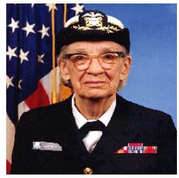
- 예시 이미지 로드
from tensorflow.keras.preprocessing.image import load_img
import numpy as np
import PIL.Image as Image
# PIL이 메모리를 더 많이 먹는다. 하지만 전처리 pil이용해서 사용할려고 pil.open한 것
# 사실은 이미지만 불러온다면 load_img를 쓰는게 더 낫다.

grace_hopper = tf.keras.utils.get_file('image.jpg','https://storage.googleapis.com/download.tensorflow.org/example_images/grace_hopper.jpg')
# grace_hopper = load_img(grace_hopper).resize(IMAGE_SHAPE)

grace_hopper = Image.open(grace_hopper).resize(IMAGE_SHAPE)
grace_hopper
- MinMax
# MinMax 해도 이미지의 정도로 표현하기 때문에 이미지가 나온다.
grace_hopper = np.array(grace_hopper)/255.0
grace_hopper.shape

# tensorhub에 있는 것
- classifier.predict
# classifier.outputs.shape
result = classifier.predict(grace_hopper[np.newaxis, ...])
type(result)
result.shape
# (1, 1001)

# argmax: 리스트 안에서 가장 큰 값의 인텍스 가져오는 것
# argsort: prediction 두번째로 큰 것
predicted_class = np.argsort(result[0], axis=-1)[-2]
predicted_class = np.argmax(result[0], axis=-1)
predicted_class
# 653

# result[0], axis=-1 안넣어도 차이가 없다.
# 653번째가 가장 크게 예측된 값이라는 것 것이다.

labels_path = tf.keras.utils.get_file('ImageNetLabels.txt','https://storage.googleapis.com/download.tensorflow.org/data/ImageNetLabels.txt')
imagenet_labels = np.array(open(labels_path).read().splitlines())
imagenet_labels[653]
# 'military uniform'
Mobilenet: 새로운 분류(꽃) 추가하기
모델(Classification) 로드 & 데이터 로드
- classification url: 모델 전체를 가져온 것 - include_top= False
# 모델 로드
classifier_url ="https://tfhub.dev/google/tf2-preview/mobilenet_v2/classification/2"
# 꽃 데이터 로드
data_root = tf.keras.utils.get_file(
  'flower_photos','https://storage.googleapis.com/download.tensorflow.org/example_images/flower_photos.tgz',
   untar=True)
- 데이터 image_generator
image_generator (flow from directory & fit_generator)
# rescale//crop/resize
image_generator = tf.keras.preprocessing.image.ImageDataGenerator(rescale=1/255)

#flow_from_directory/dataframe
# target_size= default:256
image_data = image_generator.flow_from_directory(str(data_root), target_size=IMAGE_SHAPE)
# Found 3670 images belonging to 5 classes.
for image_batch, label_batch in image_data:
    print("Image batch shape: ", image_batch.shape)
    print("Label batch shape: ", label_batch.shape)
    break
'''
Image batch shape:  (32, 224, 224, 3)
Label batch shape:  (32, 5)
'''

result_batch = classifier.predict(image_batch)
result_batch.shape
# (32, 1001)

predicted_class_names = imagenet_labels[np.argmax(result_batch, axis=-1)]
predicted_class_names.shape
# (32,)
모델(feature_extractor) 로드
-
feature url: fc(fully-connected) layer가 없습니다.
-
trainable를 False로 하게 되면 파라미터를 학습하지 않습니다.
feature_extractor_url = "https://tfhub.dev/google/tf2-preview/mobilenet_v2/feature_vector/2" #@param {type:"string"}

feature_extractor_layer = hub.KerasLayer(feature_extractor_url,
                                         input_shape=(224,224,3))

feature_batch = feature_extractor_layer(image_batch)
print(feature_batch.shape)
# (32, 1280)

feature_extractor_layer = hub.KerasLayer(feature_extractor_url,
                                         input_shape=(224,224,3))
feature_batch = feature_extractor_layer(image_batch)
print(feature_batch.shape)
# (32, 1280)

# Fit 시켰을 때 학습이 안된다.
# 모든 레이어 상속받는 애들은 trainable이 있다.
# 나중에 gan할 때 이 테크닉 잘 쓴다.
# 한쪽은 트레인 시키고, 한쪽은 트레인 안시키고 이런것들
feature_extractor_layer.trainable = False
# fc layer를 빼고 가져온다.

model = tf.keras.Sequential([
  feature_extractor_layer,
  layers.Dense(image_data.num_classes, activation='softmax')
])

model.summary()
'''
Model: "sequential_1"
_________________________________________________________________
Layer (type)                 Output Shape              Param #
=================================================================
keras_layer_2 (KerasLayer)   (None, 1280)              2257984
_________________________________________________________________
dense (Dense)                (None, 5)                 6405
=================================================================
Total params: 2,264,389
Trainable params: 6,405
Non-trainable params: 2,257,984
_________________________________________________________________
'''

predictions = model(image_batch)
model.compile(
  optimizer=tf.keras.optimizers.Adam(),
  loss='categorical_crossentropy',
  metrics=['acc'])

# 통계값 낸것
class CollectBatchStats(tf.keras.callbacks.Callback):
  def __init__(self):
    self.batch_losses = []
    self.batch_acc = []

# 배치 당 히스토리를 만들었다.
  def on_train_batch_end(self, batch, logs=None):
    self.batch_losses.append(logs['loss'])
    self.batch_acc.append(logs['acc'])
    self.model.reset_metrics()

model.summary()
'''
Model: "sequential_1"
_________________________________________________________________
Layer (type)                 Output Shape              Param #
=================================================================
keras_layer_2 (KerasLayer)   (None, 1280)              2257984
_________________________________________________________________
dense (Dense)                (None, 5)                 6405
=================================================================
Total params: 2,264,389
Trainable params: 6,405
Non-trainable params: 2,257,984
_________________________________________________________________
'''

# 에폭당 스텝별
steps_per_epoch = np.ceil(image_data.samples/image_data.batch_size)

batch_stats_callback = CollectBatchStats()

history = model.fit_generator(image_data, epochs=2,
                              steps_per_epoch=steps_per_epoch,
                             callbacks = [batch_stats_callback])
'''
Epoch 1/2
 16/115 [===>..........................] - ETA: 16:59 - loss: 0.6364 - acc: 0.7188
'''
# 학습이 오래 걸린다.
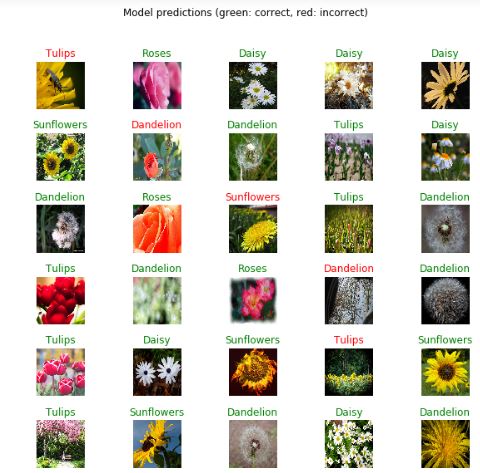
predicted_batch = model.predict(image_batch)
predicted_id = np.argmax(predicted_batch, axis=-1)
predicted_label_batch = class_names[predicted_id]

label_id = np.argmax(label_batch, axis=-1)

plt.figure(figsize=(10,9))
plt.subplots_adjust(hspace=0.5)
for n in range(30):
  plt.subplot(6,5,n+1)
  plt.imshow(image_batch[n])
  color = "green" if predicted_id[n] == label_id[n] else "red"
  plt.title(predicted_label_batch[n].title(), color=color)
  plt.axis('off')
_ = plt.suptitle("Model predictions (green: correct, red: incorrect)")
tensorflow_hub vs keras.applications
- tensorflow_hub: (장점/단점)
- 내부 구조를 알 수 없다. (자기가 만든 모델 비법을 노출하지 않을 수 있다. / 마음대로 튜닝할 수 없다.)
- 누구나 공유할 수 있다. (자기가 만든 모델{기술력} 홍보할 수 있다. / 너무 많아서 뭘 쓸지 골라야한다.)
- 고수가 활용하거나, 회사 차원에서 기술력 과시용으로 활용 가능하다.
- keras.applications: (장점/단점)
- 레이어 단위까지 내부 구조를 뽑아서 쓸 수 있다. (필요한 layer만 뽑는 등 활용성 높다. / 모델 구조 노출되므로 보안 문제가 있다.)
- 유명한 모델 몇가지만 있다. (성능 입증된 모델만 있으므로 믿을만하다. / 다양성이 부족하다. 10 정도밖에 없음)
- 초보자가 이용하기 좋다.
모델 불러오기
- hub
- feature url: fc layer가 없다.
- class url: 모델 전체를 가져온 것 include_top= False
- layer가 한개밖에 없어서 fine tuning 못한다.
- keras
- fine tuning
- 모델이 10개 밖에 없다.
## 이미지 데이터 불러오기
- numpy format
- tensor format
- 전이 학습 (Transfer learning)
○ 등장배경
사람은 task(과제) 마다 지식을 전이할 수 있는 능력이 있다 어떤 로부터 지식을 얻 고, 얻은 지식을 활용하여 그와 비슷한 task를 수행할 수 있다는 말이다 가 유사 . 할수록 지식을 전이하고 활용하기는 더욱 쉬워진다 기존의 기계학습과 . 딥러닝 알고리 즘은 고립적으로 작동하도록 고안되어있다. 이 알고리즘들은 특정한 task만 수행하도록 학습한다. 만약 feature-space( ) , 피쳐 공간 의 분포가 바뀌면 모델은 처음부터 새로 학습 해야한다. 전이학습Transfer Learning 은 배타적으로 학습하는 패러다임을 극복하고 어 떤 task로부 얻은 지식을 비슷한 task에 활용하자는 아이디어이다. Transfer Learning 의 개념과 딥러닝에서의 의의에 대해 알아보자.
데이터가 작으면 오버피팅이 생긴다. 따라서 기존에 학습했던거 가져와서 조금만 학습하면 오버피팅을 방지할 수 있다.
- Fine-tuning
1) 새로운 data set의 크기와 2) 원본 data set과의 유사도이다.
-
New data set은 작고, original data와 유사한 경우 : data가 작기 때문에 ConvNet을 과도하게 fine-tuning하는 것은 좋지 않다. New data가 original data와 유사하기 때문에 ConvNet의 상위 수준 기능이 이 new data set과 관련이 있다고 기대할 수 있다. 따라서, 마지막 linear classifier를 학습시키는 것이 좋다.
-
New data set이 크고, original data와 유사한 경우 : 더 많은 data를 보유하고 있기 때문에, 전체 network를 fine-tuning하려고 해도 괜찮다.
-
New data set은 작지만, original data와 매우 다른 경우 : data가 작기 때문에 linear classifier만 학습시키는 것이 좋다. data의 set이 매우 다르므로 더 많은 data set 관련 기능을 포함하는 classifier의 networks의 상단에서 training하는 것이 안좋다. 따라서, network의 초기 단계에서 SVM classifier를 활성화 하는 것이 더 효과적이다.
-
New data set이 크고 original data와 매우 다른 경우 : data set이 매우 크기 대문에 ConvNet을 처음 부터 교육 할 여력이 있다고 예상할 수 있다. 그러나 실제로는 pre-trained network의 weight로 초기화하는 것이 매우 유용하다.
Sequential(List)
- 라이브러리
import tensorflow as tf

import IPython.display as display
from PIL import Image
import numpy as np
import matplotlib.pyplot as plt
import os

import pathlib
- 데이터 불러오기
data_dir = tf.keras.utils.get_file(origin='https://storage.googleapis.com/download.tensorflow.org/example_images/flower_photos.tgz',
                                         fname='flower_photos', untar=True)
data_dir = pathlib.Path(data_dir)
image_count = len(list(data_dir.glob('*/*.jpg')))
image_count
# 3670
CLASS_NAMES = np.array([item.name for item in data_dir.glob('*') if item.name != "LICENSE.txt"])
CLASS_NAMES
# array(['daisy', 'dandelion', 'roses', 'sunflowers', 'tulips'],
      dtype='<U10')
- image size
for문
# for문
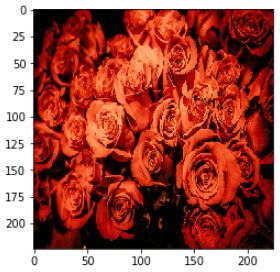
roses = list(data_dir.glob('roses/*'))
for image_path in roses[:3]:
image= Image.open(str(image_path))
image=image.resize((224,224))
plt.imshow(image)
Image_generator
# Image_generator
# The 1./255 is to convert from uint8 to float32 in range [0,1].
image_generator = tf.keras.preprocessing.image.ImageDataGenerator(rescale=1./255)
train_data_gen = image_generator.flow_from_directory(str(data_dir),
                                                    target_size=(224,224))

for image_batch, label_batch in train_data_gen:
    print("Image batch shape: ", image_batch.shape)
    print("Label batch shape: ", label_batch.shape)
    break

'''
Image batch shape:  (32, 224, 224, 3)
Label batch shape:  (32, 5)
'''
모델 불러오기 (include_top = True)
from tensorflow.keras.applications.vgg16 import VGG16
vgg16 = VGG16(include_top = True)

vgg16.summary()
'''
Model: "vgg16"
_________________________________________________________________
Layer (type)                 Output Shape              Param #
=================================================================
input_1 (InputLayer)         [(None, 224, 224, 3)]     0
_________________________________________________________________
block1_conv1 (Conv2D)        (None, 224, 224, 64)      1792
_________________________________________________________________
block1_conv2 (Conv2D)        (None, 224, 224, 64)      36928
_________________________________________________________________
block1_pool (MaxPooling2D)   (None, 112, 112, 64)      0
_________________________________________________________________
block2_conv1 (Conv2D)        (None, 112, 112, 128)     73856
_________________________________________________________________
block2_conv2 (Conv2D)        (None, 112, 112, 128)     147584
_________________________________________________________________
block2_pool (MaxPooling2D)   (None, 56, 56, 128)       0
_________________________________________________________________
block3_conv1 (Conv2D)        (None, 56, 56, 256)       295168
_________________________________________________________________
block3_conv2 (Conv2D)        (None, 56, 56, 256)       590080
_________________________________________________________________
block3_conv3 (Conv2D)        (None, 56, 56, 256)       590080
_________________________________________________________________
block3_pool (MaxPooling2D)   (None, 28, 28, 256)       0
_________________________________________________________________
block4_conv1 (Conv2D)        (None, 28, 28, 512)       1180160
_________________________________________________________________
block4_conv2 (Conv2D)        (None, 28, 28, 512)       2359808
_________________________________________________________________
block4_conv3 (Conv2D)        (None, 28, 28, 512)       2359808
_________________________________________________________________
block4_pool (MaxPooling2D)   (None, 14, 14, 512)       0
_________________________________________________________________
block5_conv1 (Conv2D)        (None, 14, 14, 512)       2359808
_________________________________________________________________
block5_conv2 (Conv2D)        (None, 14, 14, 512)       2359808
_________________________________________________________________
block5_conv3 (Conv2D)        (None, 14, 14, 512)       2359808
_________________________________________________________________
block5_pool (MaxPooling2D)   (None, 7, 7, 512)         0
_________________________________________________________________
flatten (Flatten)            (None, 25088)             0
_________________________________________________________________
fc1 (Dense)                  (None, 4096)              102764544
_________________________________________________________________
fc2 (Dense)                  (None, 4096)              16781312
_________________________________________________________________
predictions (Dense)          (None, 1000)              4097000
=================================================================
Total params: 138,357,544
Trainable params: 138,357,544
Non-trainable params: 0
_________________________________________________________________
'''
# transfer learning
# 일반적으로 학습 시간 줄어든다.
# 성능도 높여준다.
- tf.keras 라이브러리
from tensorflow.keras.layers import Dense, Flatten
from tensorflow.keras import Sequential
- transfer learning
temp = []
for layer in vgg16.layers[:4]:
    layer.trainbale = False # weights 업데이트 하느냐 안하느냐
#     featue extration: 안하는것
# fine tuning 할 대는 weights 업데이트 (자기가 골라서)
    temp.append(layer)
- fc layers 추가
temp.append(Flatten(input_shape=(None, 802816) ))

temp.append(Dense(64, activation='relu'))

temp.append(Dense(5, activation ='softmax'))

model = Sequential(temp)
model.summary()

'''
Model: "sequential_1"
_________________________________________________________________
Layer (type)                 Output Shape              Param #
=================================================================
block1_conv1 (Conv2D)        (None, 224, 224, 64)      1792
_________________________________________________________________
block1_conv2 (Conv2D)        (None, 224, 224, 64)      36928
_________________________________________________________________
block1_pool (MaxPooling2D)   (None, 112, 112, 64)      0
_________________________________________________________________
flatten_1 (Flatten)          (None, 802816)            0
_________________________________________________________________
dense_2 (Dense)              (None, 64)                51380288
_________________________________________________________________
dense_3 (Dense)              (None, 5)                 325
=================================================================
Total params: 51,419,333
Trainable params: 51,419,333
Non-trainable params: 0
_________________________________________________________________
'''
- 학습
model.compile(optimizer = tf.keras.optimizers.Adam(),
             loss='categorical_crossentropy',
             metrics=['acc'])
# one hot encoding O : categorical
model.fit_generator(train_data_gen)
모델 불러오기 (include_top = False)
include_top=False 할 시 input_shape을 맞춰줘야한다.
from tensorflow.keras.applications.vgg16 import VGG16

vgg16 = VGG16(include_top = False)

# input_shape
input1 = tensorflow.keras.layers.Input(shape=(224,224,3))
x = vgg16(input1)
x = Flatten()(x)
x = Dense(5, activation='softmax')(x)
model = tensorflow.keras.Model(inputs=input1, outputs=x)
model.summary()
'''
Model: "model_2"
_________________________________________________________________
Layer (type)                 Output Shape              Param #
=================================================================
input_7 (InputLayer)         [(None, 224, 224, 3)]     0
_________________________________________________________________
vgg16 (Model)                multiple                  14714688
_________________________________________________________________
flatten_7 (Flatten)          (None, 25088)             0
_________________________________________________________________
dense_9 (Dense)              (None, 5)                 125445
=================================================================
Total params: 14,840,133
Trainable params: 14,840,133
Non-trainable params: 0
_________________________________________________________________
'''
model.compile(optimizer = tf.keras.optimizers.Adam(),
             loss='categorical_crossentropy',
             metrics=['acc'])
# one hot encoding X : sparse_categorical
model.fit_generator(train_data_gen)
from tensorflow.keras.layers import Dense, Flatten
from tensorflow.keras import Sequential

input2 = (224,224,3)
vgg = VGG16(include_top=False,input_shape=input2)
vgg.summary()
'''
Model: "vgg16"
_________________________________________________________________
Layer (type)                 Output Shape              Param #
=================================================================
input_5 (InputLayer)         [(None, 224, 224, 3)]     0
_________________________________________________________________
block1_conv1 (Conv2D)        (None, 224, 224, 64)      1792
_________________________________________________________________
block1_conv2 (Conv2D)        (None, 224, 224, 64)      36928
_________________________________________________________________
block1_pool (MaxPooling2D)   (None, 112, 112, 64)      0
_________________________________________________________________
block2_conv1 (Conv2D)        (None, 112, 112, 128)     73856
_________________________________________________________________
block2_conv2 (Conv2D)        (None, 112, 112, 128)     147584
_________________________________________________________________
block2_pool (MaxPooling2D)   (None, 56, 56, 128)       0
_________________________________________________________________
block3_conv1 (Conv2D)        (None, 56, 56, 256)       295168
_________________________________________________________________
block3_conv2 (Conv2D)        (None, 56, 56, 256)       590080
_________________________________________________________________
block3_conv3 (Conv2D)        (None, 56, 56, 256)       590080
_________________________________________________________________
block3_pool (MaxPooling2D)   (None, 28, 28, 256)       0
_________________________________________________________________
block4_conv1 (Conv2D)        (None, 28, 28, 512)       1180160
_________________________________________________________________
block4_conv2 (Conv2D)        (None, 28, 28, 512)       2359808
_________________________________________________________________
block4_conv3 (Conv2D)        (None, 28, 28, 512)       2359808
_________________________________________________________________
block4_pool (MaxPooling2D)   (None, 14, 14, 512)       0
_________________________________________________________________
block5_conv1 (Conv2D)        (None, 14, 14, 512)       2359808
_________________________________________________________________
block5_conv2 (Conv2D)        (None, 14, 14, 512)       2359808
_________________________________________________________________
block5_conv3 (Conv2D)        (None, 14, 14, 512)       2359808
_________________________________________________________________
block5_pool (MaxPooling2D)   (None, 7, 7, 512)         0
=================================================================
Total params: 14,714,688
Trainable params: 14,714,688
Non-trainable params: 0
_________________________________________________________________
'''
tfds - cats vs. dogs
tensorflow_datasets 에는 많은 연습용 데이터들이 있습니다. 그 중 cats_vs_dogs 데이터를 불러와서 학습시켜 보도록 하겠습니다.
- 라이브러리
import os
import numpy as np
import matplotlib.pyplot as plt
import tensorflow as tf
# keras = tf.keras -> keras를 못 불러온다.
# fine tuning : keras.applications
# fine tuning X: tensorflow_hub

tf.__version__
# '2.0.0'

import tensorflow_datasets as tfds
- 데이터 불러오기
tfds.load를 통해 데이터를 불러올 수 있습니다. split 옵션을 통해서 hold_out를 해줄 수 있습니다. train_test_split은 train과 test만 나눌 수 있다면, split은 train, validation, test로 나눌 수 있습니다.
# TRAIN, VALIDATION, TEST
SPLIT_WEIGHTS = (8, 1, 1)
splits = tfds.Split.TRAIN.subsplit(weighted=SPLIT_WEIGHTS)

(raw_train, raw_validation, raw_test), metadata = tfds.load(
    'cats_vs_dogs', split=list(splits),
    with_info=True, as_supervised=True)
# with_info= True : metadata를 불러온다.
- 그래프 그려보기
# 숫자에서 string으로 바꾸는 것
get_label_name = metadata.features['label'].int2str

for image, label in raw_train.take(2):
    plt.figure()
    plt.imshow(image)
    plt.title(get_label_name(label))

- 데이터 전처리
IMG_SIZE = 160 # All images will be resized to 160x160

# resize
# 함수를 만들고, map에 넣어 준다.
def format_example(image, label):
    image = tf.cast(image, tf.float32)
    # image : [-1,1]
    # hyperbolic tangent
    image = (image/127.5) - 1
    image = tf.image.resize(image, (IMG_SIZE, IMG_SIZE))
    return image, label

train = raw_train.map(format_example)
validation = raw_validation.map(format_example)
test = raw_test.map(format_example)

# Now shuffle and batch the data.
# tfds.dataset이면 다음 기능을 쓸 수 있다.

BATCH_SIZE = 32
SHUFFLE_BUFFER_SIZE = 1000
train_batches = train.shuffle(SHUFFLE_BUFFER_SIZE).batch(BATCH_SIZE)
validation_batches = validation.batch(BATCH_SIZE)
test_batches = test.batch(BATCH_SIZE)
- MobileNet
IMG_SHAPE = (IMG_SIZE, IMG_SIZE, 3)

# Create the base model from the pre-trained model MobileNet V2
base_model = tf.keras.applications.MobileNetV2(input_shape=IMG_SHAPE,
                                               include_top=False,
                                               weights='imagenet')

# layer별로 trainable할 수 있지만, 여기서는 모델 자체를 trainable=False 해줬다.
base_model.trainable = False

base_model.summary()
# trainable_false하면 trainable params가 0이 된다. 그리고 Non-ptrainable params수가 늘어난다.
'''
Model: "mobilenetv2_1.00_160"
__________________________________________________________________________________________________
Layer (type)                    Output Shape         Param #     Connected to
==================================================================================================
input_4 (InputLayer)            [(None, 160, 160, 3) 0
__________________________________________________________________________________________________
Conv1_pad (ZeroPadding2D)       (None, 161, 161, 3)  0           input_4[0][0]
__________________________________________________________________________________________________
Conv1 (Conv2D)                  (None, 80, 80, 32)   864         Conv1_pad[0][0]
__________________________________________________________________________________________________
bn_Conv1 (BatchNormalization)   (None, 80, 80, 32)   128         Conv1[0][0]
__________________________________________________________________________________________________
Conv1_relu (ReLU)               (None, 80, 80, 32)   0           bn_Conv1[0][0]
__________________________________________________________________________________________________
expanded_conv_depthwise (Depthw (None, 80, 80, 32)   288         Conv1_relu[0][0]
__________________________________________________________________________________________________
expanded_conv_depthwise_BN (Bat (None, 80, 80, 32)   128         expanded_conv_depthwise[0][0]
__________________________________________________________________________________________________
expanded_conv_depthwise_relu (R (None, 80, 80, 32)   0           expanded_conv_depthwise_BN[0][0]
__________________________________________________________________________________________________
expanded_conv_project (Conv2D)  (None, 80, 80, 16)   512         expanded_conv_depthwise_relu[0][0
__________________________________________________________________________________________________
expanded_conv_project_BN (Batch (None, 80, 80, 16)   64          expanded_conv_project[0][0]
__________________________________________________________________________________________________
block_1_expand (Conv2D)         (None, 80, 80, 96)   1536        expanded_conv_project_BN[0][0]
__________________________________________________________________________________________________
block_1_expand_BN (BatchNormali (None, 80, 80, 96)   384         block_1_expand[0][0]
__________________________________________________________________________________________________
block_1_expand_relu (ReLU)      (None, 80, 80, 96)   0           block_1_expand_BN[0][0]
__________________________________________________________________________________________________
...
__________________________________________________________________________________________________
block_16_depthwise_BN (BatchNor (None, 5, 5, 960)    3840        block_16_depthwise[0][0]
__________________________________________________________________________________________________
block_16_depthwise_relu (ReLU)  (None, 5, 5, 960)    0           block_16_depthwise_BN[0][0]
__________________________________________________________________________________________________
block_16_project (Conv2D)       (None, 5, 5, 320)    307200      block_16_depthwise_relu[0][0]
__________________________________________________________________________________________________
block_16_project_BN (BatchNorma (None, 5, 5, 320)    1280        block_16_project[0][0]
__________________________________________________________________________________________________
Conv_1 (Conv2D)                 (None, 5, 5, 1280)   409600      block_16_project_BN[0][0]
__________________________________________________________________________________________________
Conv_1_bn (BatchNormalization)  (None, 5, 5, 1280)   5120        Conv_1[0][0]
__________________________________________________________________________________________________
out_relu (ReLU)                 (None, 5, 5, 1280)   0           Conv_1_bn[0][0]
==================================================================================================
Total params: 2,257,984
Trainable params: 0
Non-trainable params: 2,257,984
__________________________________________________________________________________________________
'''
- 모델 만들기
fc layers로 연결해주기 위해서는 데이터를 flatten해주어야 합니다.
Dense를 많이 만들지 않더라도 features가 잘 뽑혔다면 성능이 좋게 나옵니다. 즉, fealture extraction이 잘되어있다면, fc 레이어 굳이 많이 쌓을 필요 없습니다. (많아봤자 2개)
# 공간적 정보를 잃어버린다.
flatten = tf.keras.layers.Flatten()
prediction_dense = tf.keras.layers.Dense(1, activation ='sigmoid')
# sigmoid 안쓰면 regression 개념으로 쓰기 때문에 실수값으로 나온다.

model = tf.keras.Sequential([
  base_model,
  flatten,
  prediction_dense
])

model.compile(optimizer='adam',
              loss='binary_crossentropy',
              metrics=['accuracy'])

model.summary()
'''
Model: "sequential_37"
_________________________________________________________________
Layer (type)                 Output Shape              Param #
=================================================================
mobilenetv2_1.00_160 (Model) (None, 5, 5, 1280)        2257984
_________________________________________________________________
flatten_15 (Flatten)         (None, 32000)             0
_________________________________________________________________
dense_36 (Dense)             (None, 1)                 32001
=================================================================
Total params: 2,289,985
Trainable params: 32,001
Non-trainable params: 2,257,984
_________________________________________________________________
'''

model.fit(train_batches, epochs=1)
'''
- 1056s 3s/step - loss: 0.2952 - accuracy: 0.928 - 1059s 3s/step - loss: 0.2955 - accuracy: 0.928 - 1061s 3s/step - loss: 0.2950 - accuracy: 0.927 - 1064s 3s/step - loss: 0.2948 - accuracy: 0.928 - 1066s 3s/step - loss: 0.2957 - accuracy: 0.927 - 1069s 3s/step - loss: 0.2950 - accuracy: 0.928 - 1072s 3s/step - loss: 0.2953 - accuracy: 0.928 - 1074s 3s/step - loss: 0.2954 - accuracy: 0.928 - 1077s 3s/step - loss: 0.2954 - accuracy: 0.928 - 1079s 3s/step - loss: 0.2953 - accuracy: 0.928 - 1082s 3s/step - loss: 0.2959 - accuracy: 0.927 - 1085s 3s/step - loss: 0.2951 - accuracy: 0.928 - 1088s 3s/step - loss: 0.2949 - accuracy: 0.928 - 1090s 3s/step - loss: 0.2951 - accuracy: 0.928 - 1093s 3s/step - loss: 0.2950 - accuracy: 0.928 - 1096s 3s/step - loss: 0.2955 - accuracy: 0.928 - 1099s 3s/step - loss: 0.2962 - accuracy: 0.928 - 1101s 3s/step - loss: 0.2968 - accuracy: 0.928 - 1104s 3s/step - loss: 0.2968 - accuracy: 0.928 - 1104s 3s/step - loss: 0.2968 - accuracy: 0.9280
'''
GlobalAveragePooling2D
Flatten 대신 GlobalAverage(Max)Pooling을 사용할 수 있습니다.
GlobalAveragePooling은 Pooling 한 값을 평균잡아서 flatten해줍니다. 따라서 공강적 정보를 잃어버리지 않습니다.
- global average pooling
- global max pooling
global_average_layer = tf.keras.layers.GlobalAveragePooling2D()
- model 만들기
model = tf.keras.Sequential([
    base_model,
#     2차원으로 만들어준다.
    global_average_layer,
#     기계학습은 2차원
    prediction_layer
])

model.summary()
'''
Model: "sequential_44"
_________________________________________________________________
Layer (type)                 Output Shape              Param #
=================================================================
mobilenetv2_1.00_160 (Model) (None, 5, 5, 1280)        2257984
_________________________________________________________________
global_average_pooling2d_1 ( (None, 1280)              0
_________________________________________________________________
dense_28 (Dense)             (None, 1)                 1281
=================================================================
Total params: 2,259,265
Trainable params: 1,281
Non-trainable params: 2,257,984
_________________________________________________________________
'''

model.compile(optimizer='adam',
              loss='binary_crossentropy',
              metrics=['accuracy'])
model.fit(train_batches, epochs =1 )
'''
  181/Unknown - 477s 3s/step - loss: 0.2660 - accuracy: 0.89 - 480s 3s/step - loss: 0.2651 - accuracy: 0.89 - 483s 3s/step - loss: 0.2646 - accuracy: 0.89 - 486s 3s/step - loss: 0.2637 - accuracy: 0.89 - 489s 3s/step - loss: 0.2629 - accuracy: 0.89 - 492s 3s/step - loss: 0.2625 - accuracy: 0.89 - 495s 3s/step - loss: 0.2625 - accuracy: 0.89 - 495s 3s/step - loss: 0.2625 - accuracy: 0.8924 ....
'''
Comments