
본 과정은 제가 파이썬 수업을 들으면서 배운 내용을 복습하는 과정에서 적어본 것입니다.
틀린 부분이 있다면 댓글에 남겨주시면 고치도록 하겠습니다.
확실하지 않은 내용은 ‘(?)’을 함께 적었으니 그 내용을 아신다면 댓글에 남겨주시면 감사하겠습니다.
2019년 11월 21일
데이터 분석
iris
대표적인 데이터 분석 예시인 iris를 살표보도록 하겠습니다.
- iris 데이터 불러오기
import seaborn as sns
iris = sns.load_dataset('iris')
iris.head()

iris.info()
'''
<class 'pandas.core.frame.DataFrame'>
RangeIndex: 150 entries, 0 to 149
Data columns (total 5 columns):
sepal_length    150 non-null float64
sepal_width     150 non-null float64
petal_length    150 non-null float64
petal_width     150 non-null float64
species         150 non-null object
dtypes: float64(4), object(1)
memory usage: 5.9+ KB
'''

from sklearn.datasets import load_iris
data = load_iris()
data.keys()
# dict_keys(['data', 'target', 'target_names', 'DESCR', 'feature_names', 'filename'])

import pandas as pd
iris2 = pd.DataFrame(data.data, columns = data.feature_names)
iris2.head()

iris2_ta = pd.DataFrame(data.target)
iris.describe()
'''
	sepal_length	sepal_width	petal_length	petal_width
count	150.000000	150.000000	150.000000	150.000000
mean	5.843333	3.057333	3.758000	1.199333
std	0.828066	0.435866	1.765298	0.762238
min	4.300000	2.000000	1.000000	0.100000
25%	5.100000	2.800000	1.600000	0.300000
50%	5.800000	3.000000	4.350000	1.300000
75%	6.400000	3.300000	5.100000	1.800000
max	7.900000	4.400000	6.900000	2.500000
'''

sns.pairplot(iris, hue='species')
iris.skew() # 왜도
'''
sepal_length    0.314911
sepal_width     0.318966
petal_length   -0.274884
petal_width    -0.102967
dtype: float64
'''
iris.kurt() # 첨도
'''
sepal_length   -0.552064
sepal_width     0.228249
petal_length   -1.402103
petal_width    -1.340604
dtype: float64
'''

sns.heatmap(iris.corr()) # 상관분석
- 기계학습을 하기 위해서 iris 데이터 dataframe에 만들기
from sklearn.datasets import load_iris
data = load_iris()

import pandas as pd
iris_x = pd.DataFrame(data.data, columns = data.feature_names)
iris_y = pd.DataFrame(data.target, columns=['target'])
iris = pd.concat([iris_x,iris_y], axis=1)
iris.head()
'''
	sepal length (cm)	sepal width (cm)	petal length (cm)	petal width (cm)	target
0	5.1	3.5	1.4	0.2	0
1	4.9	3.0	1.4	0.2	0
2	4.7	3.2	1.3	0.2	0
3	4.6	3.1	1.5	0.2	0
4	5.0	3.6	1.4	0.2	0
'''
- Scale
스케일은 자료 집합에 적용되는 전처리 과정으로 모든 자료에 선형 변환을 적용하여 전체 자료의 분포를 평균 0, 분산 1이 되도록 만드는 과정입니다.스케일링은 자료의 오버플로우(overflow)나 언더플로우(underflow)를 방지하고 독립 변수의 공분산 행렬의 조건수(condition number)를 감소시켜 최적화 과정에서의 안정성 및 수렴 속도를 향상시킵니다.
scikit-learn에서는 다음과 같은 스케일링 클래스를 제공한다.
StandardScaler(X): 평균이 0과 표준편차가 1이 되도록 변환.
RobustScaler(X): 중앙값(median)이 0, IQR(interquartile range)이 1이 되도록 변환
MinMaxScaler(X): 최대값이 각각 1, 최소값이 0이 되도록 변환
MaxAbsScaler(X): 0을 기준으로 절대값이 가장 큰 수가 1또는 -1이 되도록 변환
- 데이터에 맞는 Specific 한 모델 찾기
기존 메트릭스 기반으로 모델 찾는 것으로 성능 체크하는데, 최적화 되어 있다.
데이터가 충분하지 않을때 교차 검증을 사용한다. 데이터가 부족하면 오버피팅 생긴다. 클로스 벨링데이션은 오버피팅을 방지하기 위해서 쓰는 것이다. holdout 시키기가 어려울 때도 cross_validate를 쓴다. 대표성을 확보하기 위해 쓴다.
큰수의 법칙에 의해서 분포에 비슷하게 간다.
cross_validation이 시간이 오래걸려서 데이터 크면 쓰기가 어려운데, 공모전 나가면 시간 없어서 못했다고 하지말고! 우리가 가진 데이터가 대표성을 띄었기 때문에 cross_validation안하고 holdout을 썼다고 말하는게 이상적
grid_search_cv
- grid: 모든 점을 다 사용했다는 것 (Ex.meshgrid ,ogrid, mgrid)
- 따로 따로 다 연산시킬 수 있다.
- cross validation
모델 찾고, 모델의 하이퍼파라미터를 찾도록 도와줍니다. 전체 데이터갖고 학습시키는 것으로 voting (ensemble) 쓰기 전에 확인하기 위해 쓰는 기법입니다. (확인 용도)
import mglearn
mglearn.plot_cross_validation.plot_group_kfold()
from sklearn.model_selection import cross_val_score, cross_val_predict, cross_validate
- cross_val_score
교차 검증을 통해 얻은 정확도를 보여줍니다.
from sklearn.neighbors import KNeighborsClassifier
knn = KNeighborsClassifier()
cross_val_score(KNeighborsClassifier(), iris.iloc[:,:-1], iris.target, cv=10)
'''
array([1.        , 0.93333333, 1.        , 1.        , 0.86666667,
       0.93333333, 0.93333333, 1.        , 1.        , 1.        ])
'''
- GridSearchCV
모델의 최적의 하이퍼파라미터를 찾고자할 때 씁니다. 보통 모델링의 하이퍼 파라미터를 확인해보고 싶다면, (예시: KNN) vars(knn) 또는 knn.get_params()를 통해 하이퍼 파라미터를 확인합니다.
from sklearn.model_selection import GridSearchCV

## knn
vars(knn) # 값이 변할 때 체크를 할 수 있다.
'''
{'n_neighbors': 5,
 'radius': None,
 'algorithm': 'auto',
 'leaf_size': 30,
 'metric': 'minkowski',
 'metric_params': None,
 'p': 2,
 'n_jobs': None,
 'weights': 'uniform'}
'''

knn.get_params()
'''
{'algorithm': 'auto',
 'leaf_size': 30,
 'metric': 'minkowski',
 'metric_params': None,
 'n_jobs': None,
 'n_neighbors': 5,
 'p': 2,
 'weights': 'uniform'}
'''

clf = GridSearchCV(knn, {'n_neighbors':[1,10,20], 'leaf_size':[20,30,40]}, cv=10)
clf.fit(iris.iloc[:,:-1],iris.target)
'''
GridSearchCV(cv=10, error_score='raise-deprecating',
       estimator=KNeighborsClassifier(algorithm='auto', leaf_size=30, metric='minkowski',
           metric_params=None, n_jobs=None, n_neighbors=5, p=2,
           weights='uniform'),
       fit_params=None, iid='warn', n_jobs=None,
       param_grid={'n_neighbors': [1, 10, 20], 'leaf_size': [20, 30, 40]},
       pre_dispatch='2*n_jobs', refit=True, return_train_score='warn',
       scoring=None, verbose=0)
'''

clf.best_params_
# {'leaf_size': 20, 'n_neighbors': 20}

pd.DataFrame(clf.cv_results_).T
'''

0	1	2	3	4	5	6	7	8
mean_fit_time	0.00289819	0.00239851	0.00259855	0.00279846	0.00269845	0.00229859	0.00219867	0.00499685	0.00239859
std_fit_time	0.00113453	0.000489814	0.000490097	0.000399781	0.000458012	0.000458048	0.000399364	0.00236523	0.000489658
mean_score_time	0.00329754	0.00269849	0.00289872	0.00229881	0.00269825	0.00279837	0.00299845	0.00389776	0.00279799
std_score_time	0.000780019	0.000458043	0.000943091	0.000457804	0.000457886	0.000399793	0.000447235	0.000830224	0.00039984
param_leaf_size	20	20	20	30	30	30	40	40	40
param_n_neighbors	1	10	20	1	10	20	1	10	20
params	{'leaf_size': 20, 'n_neighbors': 1}	{'leaf_size': 20, 'n_neighbors': 10}	{'leaf_size': 20, 'n_neighbors': 20}	{'leaf_size': 30, 'n_neighbors': 1}	{'leaf_size': 30, 'n_neighbors': 10}	{'leaf_size': 30, 'n_neighbors': 20}	{'leaf_size': 40, 'n_neighbors': 1}	{'leaf_size': 40, 'n_neighbors': 10}	{'leaf_size': 40, 'n_neighbors': 20}
split0_test_score	1	1	1	1	1	1	1	1	1
split1_test_score	0.933333	0.933333	0.933333	0.933333	0.933333	0.933333	0.933333	0.933333	0.933333
split2_test_score	1	1	1	1	1	1	1	1	1
split3_test_score	0.933333	1	1	0.933333	1	1	0.933333	1	1
split4_test_score	0.866667	1	1	0.866667	1	1	0.866667	1	1
split5_test_score	1	0.866667	0.933333	1	0.866667	0.933333	1	0.866667	0.933333
split6_test_score	0.866667	0.933333	0.933333	0.866667	0.933333	0.933333	0.866667	0.933333	0.933333
split7_test_score	1	0.933333	1	1	0.933333	1	1	0.933333	1
split8_test_score	1	1	1	1	1	1	1	1	1
split9_test_score	1	1	1	1	1	1	1	1	1
mean_test_score	0.96	0.966667	0.98	0.96	0.966667	0.98	0.96	0.966667	0.98
std_test_score	0.0533333	0.0447214	0.0305505	0.0533333	0.0447214	0.0305505	0.0533333	0.0447214	0.0305505
rank_test_score	7	4	1	7	4	1	7	4	1
split0_train_score	1	0.97037	0.977778	1	0.97037	0.977778	1	0.97037	0.977778
split1_train_score	1	0.985185	0.985185	1	0.985185	0.985185	1	0.985185	0.985185
split2_train_score	1	0.977778	0.962963	1	0.977778	0.962963	1	0.977778	0.962963
split3_train_score	1	0.977778	0.977778	1	0.977778	0.977778	1	0.977778	0.977778
split4_train_score	1	0.977778	0.977778	1	0.977778	0.977778	1	0.977778	0.977778
split5_train_score	1	0.97037	0.977778	1	0.97037	0.977778	1	0.97037	0.977778
split6_train_score	1	0.985185	0.985185	1	0.985185	0.985185	1	0.985185	0.985185
split7_train_score	1	0.977778	0.977778	1	0.977778	0.977778	1	0.977778	0.977778
split8_train_score	1	0.977778	0.977778	1	0.977778	0.977778	1	0.977778	0.977778
split9_train_score	1	0.962963	0.940741	1	0.962963	0.940741	1	0.962963	0.940741
mean_train_score	1	0.976296	0.974074	1	0.976296	0.974074	1	0.976296	0.974074
std_train_score	0	0.00645763	0.0125051	0	0.00645763	0.0125051	0	0.00645763	0.0125051
'''
Randomized Search CV (시간 없을 때 돌리기엔 좋다.)
- Pipeline
pipeline/estimator
gird search cv에 파이프라인을 넣을 수 있습니다.
from sklearn.pipeline import Pipeline, make_pipeline
from sklearn.preprocessing import StandardScaler

pipe = make_pipeline(StandardScaler(), KNeighborsClassifier())
pipe = Pipeline([('ss', StandardScaler()),('knn',KNeighborsClassifier())])
pipe.fit(iris.iloc[:,:-1], iris.target)
'''
Pipeline(memory=None,
     steps=[('ss', StandardScaler(copy=True, with_mean=True, with_std=True)), ('knn', KNeighborsClassifier(algorithm='auto', leaf_size=30, metric='minkowski',
           metric_params=None, n_jobs=None, n_neighbors=5, p=2,
           weights='uniform'))])
'''

vars(pipe)
'''
{'steps': [('ss', StandardScaler(copy=True, with_mean=True, with_std=True)),
  ('knn',
   KNeighborsClassifier(algorithm='auto', leaf_size=30, metric='minkowski',
              metric_params=None, n_jobs=None, n_neighbors=5, p=2,
              weights='uniform'))],
 'memory': None}
'''

# Mangling 이름앞에 __
# list로 묶어서 동시에 여러개 테크닉을 집어 넣을 수도 있다.
clf = GridSearchCV(pipe, [{'knn__n_neighbors':[1,10], 'knn__leaf_size':[20,30]}], cv=10)

clf.fit(iris.iloc[:,:-1], iris.target)
'''
GridSearchCV(cv=10, error_score='raise-deprecating',
       estimator=Pipeline(memory=None,
     steps=[('ss', StandardScaler(copy=True, with_mean=True, with_std=True)), ('knn', KNeighborsClassifier(algorithm='auto', leaf_size=30, metric='minkowski',
           metric_params=None, n_jobs=None, n_neighbors=5, p=2,
           weights='uniform'))]),
       fit_params=None, iid='warn', n_jobs=None,
       param_grid={'knn__n_neighbors': [1, 10], 'knn__leaf_size': [20, 30]},
       pre_dispatch='2*n_jobs', refit=True, return_train_score='warn',
       scoring=None, verbose=0)
'''
- DummyClassifier
 from sklearn.dummy import DummyClassifier
 du = DummyClassifier()
# most_frequent: 70:30 -> 많이 있는 데이터라도 맞추자 해서 70을 더 많이 보는 것
# imbalance 데이터셋 99:1 -> 99% 이상이 나오도록 한다.

pipe = Pipeline([('std', StandardScaler()), ('clf', DummyClassifier())])
# clf 를 아무거나 넣고, 나중에 gridsearchcv할 때 알고리즘을 바꿔도 할 수 있다.
# 알고리즘 / 하이퍼파라미터 함께 만들어서 데이터를 돌려보면 된다.
# 파이프라인 / 전처리
# 꼼수...

param_gird = [
    {'clf':[LogisticRegression()], 'clf__C':[1.,2.,3.]},
    {'clf':[KNeighborsClassifier()], 'clf__n_neighbors':[1,2,3]}
]

gird = GridSearchCV(pipe, param_grid, cv =kf )

grid.fit(wine_data.iloc[:,:-1], wine_data.target)
'''
GridSearchCV(cv=StratifiedKFold(n_splits=10, random_state=None, shuffle=False),
             error_score='raise-deprecating',
             estimator=Pipeline(memory=None,
                                steps=[('standardscaler',
                                        StandardScaler(copy=True,
                                                       with_mean=True,
                                                       with_std=True)),
                                       ('stackingclassifier',
                                        StackingClassifier(average_probas=False,
                                                           classifiers=[RandomForestClassifier(bootstrap=True,
                                                                                               class_weight=Non...
                                                                                              warm_start=False),
                                                           store_train_meta_features=False,
                                                           use_clones=True,
                                                           use_features_in_secondary=False,
                                                           use_probas=False,
                                                           verbose=0))],
                                verbose=False),
             iid='warn', n_jobs=None,
             param_grid={'stackingclassifier__kneighborsclassifier__n_neighbors': [1,
                                                                                   2,
                                                                                   3,
                                                                                   4,
                                                                                   5],
                         'stackingclassifier__svc__C': [1, 2, 3]},
             pre_dispatch='2*n_jobs', refit=True, return_train_score=False,
             scoring=None, verbose=0)
'''

grid.best_params_
'''
{'stackingclassifier__kneighborsclassifier__n_neighbors': 3,
 'stackingclassifier__svc__C': 1}
'''
clf3= GridSearchCV(pipe, [{'clf': [DummyClassifier()], 'clf__strategy':['most_frequent','stratified']},
                          {'clf': [KNeighborsClassifier()], 'clf__n_neighbors':[ i for i in range(2,10)]}], cv=10)

clf3.fit(iris.iloc[:,:-1], iris.target)
'''
GridSearchCV(cv=10, error_score='raise-deprecating',
       estimator=Pipeline(memory=None,
     steps=[('clf', DummyClassifier(constant=None, random_state=None, strategy='stratified'))]),
       fit_params=None, iid='warn', n_jobs=None,
       param_grid=[{'clf': [DummyClassifier(constant=None, random_state=None, strategy='stratified')], 'clf__strategy': ['most_frequent', 'stratified']}, {'clf': [KNeighborsClassifier(algorithm='auto', leaf_size=30, metric='minkowski',
           metric_params=None, n_jobs=None, n_neighbors=9, p=2,
           weights='uniform')], 'clf__n_neighbors': [2, 3, 4, 5, 6, 7, 8, 9]}],
       pre_dispatch='2*n_jobs', refit=True, return_train_score='warn',
       scoring=None, verbose=0)
'''

clf3.best_params_
'''
{'clf': KNeighborsClassifier(algorithm='auto', leaf_size=30, metric='minkowski',
            metric_params=None, n_jobs=None, n_neighbors=9, p=2,
            weights='uniform'), 'clf__n_neighbors': 9}
'''
- KFold
from sklearn.model_selection import KFold
kf = KFold(10, shuffle=True)
# random 하기 뽑아서: shuffle
t = kf.split(data.iloc[:,:-1], data.target)
next(t)
'''
(array([  2,   3,   4,   5,   6,   7,   8,   9,  10,  11,  12,  13,  14,
         16,  17,  18,  19,  20,  21,  22,  23,  24,  25,  26,  27,  28,
         29,  30,  31,  32,  33,  34,  35,  36,  37,  38,  40,  41,  42,
         43,  44,  45,  46,  47,  49,  50,  51,  52,  53,  54,  55,  56,
         58,  59,  60,  61,  62,  63,  64,  65,  66,  67,  68,  70,  71,
         72,  73,  75,  76,  77,  78,  79,  80,  81,  83,  84,  85,  86,
         87,  88,  89,  90,  91,  92,  93,  94,  95,  96,  97,  98,  99,
        100, 101, 102, 103, 104, 105, 106, 107, 108, 109, 110, 111, 112,
        113, 114, 115, 116, 117, 119, 120, 121, 122, 123, 124, 125, 126,
        127, 128, 129, 130, 131, 132, 133, 134, 135, 136, 138, 139, 140,
        141, 142, 143, 145, 146, 147, 148, 149, 150, 151, 152, 153, 154,
        155, 156, 158, 159, 160, 162, 163, 164, 165, 166, 167, 169, 171,
        172, 174, 176, 177]),
 array([  0,   1,  15,  39,  48,  57,  69,  74,  82, 118, 137, 144, 157,
        161, 168, 170, 173, 175]))
'''
- StratifiedKFold
층화계층법으로 출력변수가 범주형일 경우 클래스 등분 비율에 맞춰서 쪼개줍니다. train_test_split에서도 stratify를 설정해주면 자동으로 클래스에 맞게 쪼개줍니다.
from sklearn.model_selection import StratifiedKFold
# 층화계층법
kf2 = StratifiedKFold(10)
cross_val_score(KNeighborsClassifier(),
               data.iloc[:,:-1], data.target, cv = kf2).var()
- ShuffleSplit
from sklearn.model_selection import ShuffleSplit
ss = ShuffleSplit()
ss.split(data.iloc[:,:-1], data.target)
for a,b in ss.split(data.iloc[:,:-1], data.target):
    print(b)
'''
[ 63  77  22 176  29  41 145  26  43  16  78 127  96  11  56  68 140 134]
[148  17  12 130  36  37  30 102  39   6  23 121 153  50 108  55 139   7]
[ 70  84  40 121  98  47 170  69  99  35  51  73  30  33  95 104 127  16]
[ 39 169  65 111 164  82  42  93 151  21 150 157 172 168 109  69   7  38]
[ 65  19  92  54 107  13  11 170 124 125   6   2   9  16 129 123 155  46]
[138  39 136  66 139 113 141  52  13 168  18 173  38  90 108   8  17  86]
[118   5 170  12  22  59  33  19 176 175  48  44   2  70 151 140 117 134]
[173 160  13 138  84   2  93   9 105  95  81 164 118  87  17 110  56  53]
[  6 129 128 115 136  97   9 162 165  53   4 112 176 160  72 175  12 134]
[ 71 121  63 137  36  62 128  93  31 113   9  61  33 101 133  41  42 130]
'''
cross_val_score(KNeighborsClassifier(),
               data.iloc[:,:-1], data.target, cv = ss).var()
# 0.018395061728395057
Auto ML
from tpot import TPOTClassifier
tp = TPOTClassifier(10,10)

tp.fit(iris.iloc[:,:-1], iris.target)
# xgboost 까지 합쳐서 만들어준다.
'''
TPOTClassifier(config_dict=None, crossover_rate=0.1, cv=5,
        disable_update_check=False, early_stop=None, generations=10,
        max_eval_time_mins=5, max_time_mins=None, memory=None,
        mutation_rate=0.9, n_jobs=1, offspring_size=None,
        periodic_checkpoint_folder=None, population_size=10,
        random_state=None, scoring=None, subsample=1.0, template=None,
        use_dask=False, verbosity=0, warm_start=False)
'''

tp.export('tp.py')
# 최적의 알고리즘과 하이퍼파라미터를 py로 저장해준다.
Feature Selection
Filter, Wrapper, Embedded 방식 (feature selection)
- Filter: 통계 방법 (feature importance)
- Wrapper: 기계학습과 동시에 해서 backward를 통해 찾는 방법
- SelectKBest
Filter 방식으로 유의미한 변수들을 고르는 기법입니다.
from sklearn.feature_selection import SelectKBest, chi2
# filter method
skb = SelectKBest(chi2, 2)

skb.fit_transform(iris.iloc[:,:-1], iris.target)[:5]
# 카이제곱 기준으로 가장 좋은 변수들을 뽑아낸다.
'''
array([[1.4, 0.2],
       [1.4, 0.2],
       [1.3, 0.2],
       [1.5, 0.2],
       [1.4, 0.2]])
'''
skb.get_support()
# array([False, False,  True,  True])
vars(skb)
'''
{'score_func': <function sklearn.feature_selection.univariate_selection.chi2(X, y)>,
 'k': 2,
 'scores_': array([ 10.81782088,   3.7107283 , 116.31261309,  67.0483602 ]),
 'pvalues_': array([4.47651499e-03, 1.56395980e-01, 5.53397228e-26, 2.75824965e-15])}
'''
- RFE
Wrapper 방식으로 유의미한 변수들을 뽑는 기법입니다.
from sklearn.feature_selection import RFE
# wrapper method
from sklearn.ensemble import RandomForestClassifier

rfe = RFE(RandomForestClassifier(),3) # recursive feature elimination
# 변수를 한개빼고, 한개빼면서 보여주는 것
# 차원의 저주
# RandomForest을 써서 4개 변수를 줄이는 것

rfe.fit_transform(iris.iloc[:,:-1], iris.target)[:5]
'''
array([[5.1, 1.4, 0.2],
       [4.9, 1.4, 0.2],
       [4.7, 1.3, 0.2],
       [4.6, 1.5, 0.2],
       [5. , 1.4, 0.2]])
'''
rfe.get_support()
# array([ True, False,  True,  True])
vars(rfe)
'''
{'estimator': RandomForestClassifier(bootstrap=True, class_weight=None, criterion='gini',
             max_depth=None, max_features='auto', max_leaf_nodes=None,
             min_impurity_decrease=0.0, min_impurity_split=None,
             min_samples_leaf=1, min_samples_split=2,
             min_weight_fraction_leaf=0.0, n_estimators='warn', n_jobs=None,
             oob_score=False, random_state=None, verbose=0,
             warm_start=False),
 'n_features_to_select': 3,
 'step': 1,
 'verbose': 0,
 'estimator_': RandomForestClassifier(bootstrap=True, class_weight=None, criterion='gini',
             max_depth=None, max_features='auto', max_leaf_nodes=None,
             min_impurity_decrease=0.0, min_impurity_split=None,
             min_samples_leaf=1, min_samples_split=2,
             min_weight_fraction_leaf=0.0, n_estimators=10, n_jobs=None,
             oob_score=False, random_state=None, verbose=0,
             warm_start=False),
 'n_features_': 3,
 'support_': array([ True, False,  True,  True]),
 'ranking_': array([1, 2, 1, 1])}
'''
# 최적화된 변수 개수 어떻게 뽑지? - 실험적으로 ...
# 데이터로부터 최적의 모델 찾는 것
PCA
feature selection은 변수를 줄이지만, PCA는 차원을 줄이지만 특성은 그대로 갖고 있다.
from sklearn.decomposition import PCA
pca = PCA(3)
# 요즘에는 많이 안쓴다.
# 영상처리에서는 많이 쓴다.
pca.fit_transform(iris.iloc[:,:-1])
# 모든 값을 바꿔주는 특징이 있다.
'''
array([[-2.68,  0.32, -0.03],
       [-2.71, -0.18, -0.21],
       [-2.89, -0.14,  0.02],
       [-2.75, -0.32,  0.03],
       [-2.73,  0.33,  0.09]])
'''
vars(pca)
'''
{'n_components': 3,
 'copy': True,
 'whiten': False,
 'svd_solver': 'auto',
 'tol': 0.0,
 'iterated_power': 'auto',
 'random_state': None,
 '_fit_svd_solver': 'full',
 'mean_': array([5.84333333, 3.05733333, 3.758     , 1.19933333]),
 'noise_variance_': 0.023835092973449445,
 'n_samples_': 150,
 'n_features_': 4,
 'components_': array([[ 0.36138659, -0.08452251,  0.85667061,  0.3582892 ],
        [ 0.65658877,  0.73016143, -0.17337266, -0.07548102],
        [-0.58202985,  0.59791083,  0.07623608,  0.54583143]]),
 'n_components_': 3,
 'explained_variance_': array([4.22824171, 0.24267075, 0.0782095 ]),
 'explained_variance_ratio_': array([0.92461872, 0.05306648, 0.01710261]),
 'singular_values_': array([25.09996044,  6.01314738,  3.41368064])}
'''
앙상블
VotingClassifier
from sklearn.datasets import load_iris
data = load_iris()

# ensemble
from sklearn.ensemble import VotingClassifier

from sklearn.neighbors import KNeighborsClassifier
from sklearn.linear_model import LogisticRegression

vote = VotingClassifier([('KNN',KNeighborsClassifier()), ('lr',LogisticRegression())])

from sklearn.model_selection import cross_val_score
cross_val_score(vote, data.data,data.target, cv=10).mean()
# 0.9666666666666668

# Voting Classifier의 예시
'''
clf = VotingClassifier(estimators=[
        ('lr', clf1), ('rf', clf2), ('gnb', clf3)],
        voting='soft', weights=[2,1,1],
        flatten_transform=True)
'''
Bagging
Bagging은 복원 랜덤 추출을 통해 각 모델을 학습시켜 학습된 모델의 예측변수를 집계(Aggregating) 하는 방법입니다.
일반적으로 Categorical Data인 경우, 투표 방식 (Voting)으로 집계하며 Continuous Data인 경우, 평균 (Average)으로 집계합니다.
- overfitting 잘 나는 경우 (variance high)
-
장점: 성능은 비슷하게 유지하지만 overfitting을 줄일 수 있습니다. 각 샘플에서 나타난 결과를 어느정도 중간값으로 맞춰주기 때문에 overfitting을 피할 수 있습니다.
- Randomforest : decision tree가 bagging 되어 있습니다.
- 높은 bias로 인한 Underfitting
- 높은 Variance로 인한 Overfitting
BaggingClassifier
from sklearn.ensemble import BaggingClassifier

bag = BaggingClassifier(LogisticRegression(), 5)
cross_val_score(bag, data.data, data.target).mean()
# 0.9538398692810457
Boosting
Bagging이 일반적인 모델을 만드는데 집중되어있다면, Boosting은 맞추기 어려운 문제를 맞추는데 초점이 맞춰져 있습니다.
Boosting도 Bagging과 동일하게 복원 랜덤 샘플링을 하지만, 가중치를 부여한다는 차이점이 있습니다. Bagging이 병렬로 학습하는 반면, Boosting은 순차적으로 학습시킵니다. 학습이 끝나면 나온 결과에 따라 가중치가 재분배됩니다.
오답에 대해 높은 가중치를 부여하고, 정답에 대해 낮은 가중치를 부여하기 때문에 오답에 더욱 집중할 수 있게 되는 것 입니다. Boosting 기법의 경우, 정확도가 높게 나타납니다. 하지만, 그만큼 Outlier에 취약하기도 합니다.
수학 문제를 푸는데 9번 문제가 엄청 어려워서 계속 틀렸다고 가정해보겠습니다. Boosting 방식은 9번 문제에 가중치를 부여해서 9번 문제를 잘 맞춘 모델을 최종 모델로 선정합니다. 아래 그림을 통해 자세히 알아보겠습니다.
XGBoosting GradientBoost AdaBoost : Ada 계산기 만든 여자 이름 따서 만든 모델 Light GBM
AdaBoostClassifier
from sklearn.ensemble import AdaBoostClassifier

ada = AdaBoostClassifier(LogisticRegression())
cross_val_score(ada, data.data, data.target, cv =10).mean()
# 0.6666666666666667
GradientBoostingClassifier
from sklearn.ensemble import GradientBoostingClassifier
Stacking
Meta Modeling 이라고 불리기도 하는 이 방법은 위의 2가지 방식과는 조금 다릅니다. “Two heads are better than one” 이라는 아이디어에서 출발합니다.
Stacking은 서로 다른 모델들을 조합해서 최고의 성능을 내는 모델을 생성합니다. 여기에서 사용되는 모델은 SVM, RandomForest, KNN 등 다양한 알고리즘을 사용할 수 있습니다. 이러한 조합을 통해 서로의 장점은 취하고 약점을 보완할 수 있게 되는 것 입니다.
- 앙상블 설명은 다음 사이트를 참고하였습니다.
!pip install -U mlxtend
from mlxtend.classifier import StackingClassifier
from sklearn.naive_bayes import GaussianNB

stack = StackingClassifier([ada,bag, GaussianNB()], LogisticRegression())
# meta_Classifier: logistic regression을 많이 쓴다.
cross_val_score(stack, data.data, data.target, cv=10).mean()
# 0.9466666666666667
DummyClassification
Strategy :
* "stratified": generates predictions by respecting the training
  set's class distribution
* "most_frequent": always predicts the most frequent label in the
  training set.
* "prior": always predicts the class that maximizes the class prior
  (like "most_frequent") and ``predict_proba`` returns the class prior.
* "uniform": generates predictions uniformly at random.
* "constant": always predicts a constant label that is provided by
  the user. This is useful for metrics that evaluate a non-majority
  class
# 데이터 로드
from sklearn.datasets import load_wine
import pandas as pd

wine = load_wine()
wine_data = pd.DataFrame(wine.data, columns = wine.feature_names)

# SelectKBest
from sklearn.feature_selection import chi2, SelectKBest
kb = SelectKBest(chi2, 5)

# DummyClassification
from sklearn.dummy import DummyClassifier
# algorith + hyperparameter

pipe = Pipeline([('std', StandardScaler()), ('clf', DummyClassifier())])
param_gird = [
    {'clf':[LogisticRegression()], 'clf__C':[1.,2.,3.]},
    {'clf':[KNeighborsClassifier()], 'clf__n_neighbors':[1,2,3]}
]
gird = GridSearchCV(pipe, param_grid, cv =kf )
grid.fit(wine_data.iloc[:,:-1], wine_data.target)
'''
GridSearchCV(cv=StratifiedKFold(n_splits=10, random_state=None, shuffle=False),
             error_score='raise-deprecating',
             estimator=Pipeline(memory=None,
                                steps=[('standardscaler',
                                        StandardScaler(copy=True,
                                                       with_mean=True,
                                                       with_std=True)),
                                       ('stackingclassifier',
                                        StackingClassifier(average_probas=False,
                                                           classifiers=[RandomForestClassifier(bootstrap=True,
                                                                                               class_weight=Non...
                                                                                              warm_start=False),
                                                           store_train_meta_features=False,
                                                           use_clones=True,
                                                           use_features_in_secondary=False,
                                                           use_probas=False,
                                                           verbose=0))],
                                verbose=False),
             iid='warn', n_jobs=None,
             param_grid={'stackingclassifier__kneighborsclassifier__n_neighbors': [1,
                                                                                   2,
                                                                                   3,
                                                                                   4,
                                                                                   5],
                         'stackingclassifier__svc__C': [1, 2, 3]},
             pre_dispatch='2*n_jobs', refit=True, return_train_score=False,
             scoring=None, verbose=0)
'''

grid.best_params_
'''
{'stackingclassifier__kneighborsclassifier__n_neighbors': 3,
 'stackingclassifier__svc__C': 1}
'''
Model 성능 평가
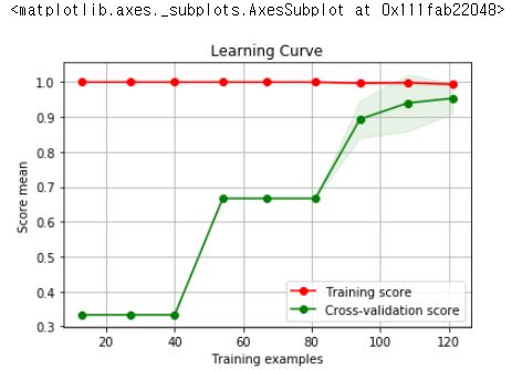
learning_curve
학습 곡선은 x축을 학습 데이터의 개수, y축을 성능 점수로 하여 학습 데이터의 양을 조금씩 늘릴 때마다 성능이 어떻게 변화하는지 보여주는 곡선입니다. 옵션 중에 train_sizes는 그래프의 간격을 의미합니다.
import numpy as np
from sklearn.model_selection import learning_curve

train_size, train_score, test_score = learning_curve(RandomForestClassifier(),iris.iloc[:,:-1],iris.target,cv=10, train_sizes=np.linspace(0.1,0.9,9))

from sklearn_evaluation import plot

plot.learning_curve(train_score, test_score, train_size)
# 데이타에 따라서 어떻게 변화는가 보는 기법
# epoch도 봐야하고, learning curve도 볼 줄 알아야한다.
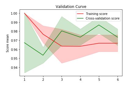
validation_curve
from sklearn.model_selection import validation_curve
train_score, test_score = validation_curve(KNeighborsClassifier(), iris.iloc[:,:-1], iris.target,
                 'n_neighbors', [1,2,3,4,5,6])
import sklearn_evaluation
sklearn_evaluation.plot.validation_curve(train_score,test_score, [1,2,3,4,5,6])
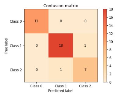
confusion_matrix
from sklearn.model_selection import train_test_split
X_train, X_test, y_train, y_test = train_test_split(iris.iloc[:,:-1], iris.iloc[:,-1])

from sklearn.metrics import confusion_matrix
confusion = confusion_matrix(y_test, rf.predict(X_test))
confusion
'''
array([[11,  0,  0],
       [ 0, 18,  1],
       [ 0,  1,  7]], dtype=int64)
'''

# 오차행렬(confusion_matrix)
plot.confusion_matrix(y_test, rf.predict(X_test))
한번 데이터 분석 해보기
data.go.kr 에서 도로교통사고 통계 데이터를 가져와서 한번 EDA 및 전처리를 해보겠습니다.
# 정부에서 나온것은 cp949로 인코딩해야합니다.
f = pd.read_csv('14일_frequencyaccident_20191010.csv', encoding = 'cp949')
Classification report
suppport는 실제 타겟 클래스의 개수입니다. 클래스별 평가 점수의 평균을 모델의 종합 성능 점수로 활용합니다. macro avg는 단순 평균, weighted avg는 각 클래스에 속하는 표본의 개수로 가중평균을 낸 것입니다.
from sklearn.metrics import classification_report
print(classification_report(y_test, rf.predict(X_test)))
'''
              precision    recall  f1-score   support

           0       1.00      1.00      1.00        11
           1       0.95      0.95      0.95        19
           2       0.88      0.88      0.88         8

    accuracy                           0.95        38
   macro avg       0.94      0.94      0.94        38
weighted avg       0.95      0.95      0.95        38

'''
무단 배포 금지
Comments